A Drained Mohr–Coulomb Soil Solver

1Introduction

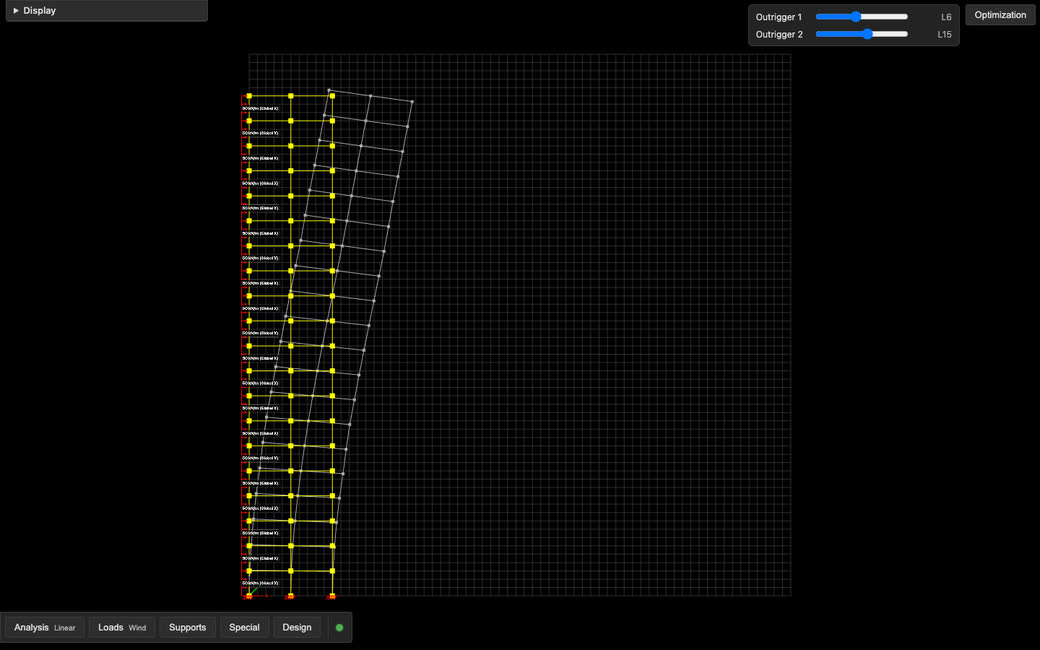
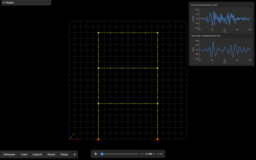
Geotechnical design is settled at the limit state: how much load the ground carries before a mechanism forms, and how far it moves on the way there. This paper describes the engine that answers both — a static, small-strain, effective-stress plane-strain finite element solver, elastic–perfectly-plastic Mohr–Coulomb at every integration point, driven by Newton–Raphson to collapse rather than stopping short of it, with layered ground, a phreatic line, a K₀ initial state and staged excavation on top, and retaining walls with Coulomb soil–wall interfaces and struts. It is the first four stages of a solver for braced excavation analysis, each of the last three boundary conditions and bookkeeping on the core rather than a change to it.

Because everything downstream inherits its errors, the core is verified three ways: against closed forms, against a mesh refinement sequence whose limit is known, and — because no closed form separates discretisation error from a bug in the constitutive code — against an independent open-source solver on the same element and the same mesh. It reaches 1.0493 times the exact Prandtl load, approaching from above as a displacement-based upper bound must, and agrees with OpenGeoSys to 2.15 × 10^-5 in displacement where either code differs from the closed form by tens of percent.

2Theory

Plane strain fixes the out-of-plane strains at zero but not the out-of-plane stress, and Mohr–Coulomb responds to all three principal stresses — out of plane is frequently the intermediate one, the reason plane strain mobilises more strength than a triaxial test. σ′_zz is therefore integrated as a fourth state component rather than recovered from the in-plane pair. All stress is effective and tension-positive, in the API as well as the internals, with pore pressure — prescribed by a phreatic line, hydrostatic below it and no suction above — entering only as an external load. A construction phase declares everything that acts in it and inherits the previous phase’s stress; the solver ramps the difference, so self-weight and a water table carry across phases and a lowered water table is a load like any other. The initial state comes from gravity loading or from the K₀ procedure, which prescribes the lateral stress from the overburden and each layer’s K₀ under the same horizontal-ground restriction Plaxis places on it. Excavation is the same rule applied to which elements exist: every integral runs over the active elements, so leaving soil out of a phase removes its stiffness, its weight and its stress, and what the phase ramps is the force that soil exerted on what remains. The water standing on any exposed boundary is applied automatically from the phreatic line on its far side — the excavated cluster’s own, so a pit left on the water table is flooded and one given a lower line is dry — and a dewatered pit under a retained table then carries the unbalanced water load a retaining wall exists for. The wall is Plaxis’s plate, a three-node Mindlin beam on an element edge with a rotation at each node, and the soil on either face meets it through a zero-thickness Coulomb interface integrated at its node pairs: elastic until the shear reaches R_inter times the adjacent soil’s strength, opening under the tension cut-off with a gap that must close before it bears again. The interface works in effective stress; the soil face along it carries its own water like any exposed boundary, and the wall receives the equal and opposite traction from each side, so two sides under different water levels leave the wall with the unbalanced load. An uninstalled wall’s line is continuous soil — its node pairs are tied — and installing it releases the tie and ramps the earth pressure onto the interface by the same phase rule that excavates. Struts are bars that carry what moves after they exist; prestress is a force imposed during a phase and held as the strut’s own from the next.

The element is the six-node triangle: quadratic displacement, hence linear strain, at three Gauss points; the constant-strain alternative is too stiff for the bending-dominated wall problems this solver is aimed at. Stress, plastic strain and the yield flag live at the integration points, and nodal values are recovered by exact extrapolation rather than a fit.

Mohr–Coulomb is used in its full hexagonal form, written as six yield functions — the permutations of the principal stresses — so no advance knowledge of their ordering is needed, with a tension cut-off because the bare pyramid would carry isotropic tension all the way to its apex, which is wrong behind a retaining wall. The return mapping is performed in principal stress space by the closed-form algorithm of Clausen, Damkilde and Andersen, which turns the hexagon’s edges and apex into explicit regions rather than corners to be negotiated with active-set logic.

Flow is non-associated: the plastic potential is built on the dilation angle, which is not optional for soil, where associated flow grossly overpredicts both dilation and collapse load. It costs symmetry — the consistent tangent implied by the return map, eigenbasis rotation included, is non-symmetric, so the sparse global system is factorised with a general LU rather than a Cholesky. Newton–Raphson drives it, bisecting any increment that fails to converge and carrying per-integration-point history in and out, so a later construction phase starts where the previous one finished.

3Benchmarks

The reference problem is a rigid strip footing on weightless cohesive soil, pushed to collapse under displacement control; its exact limit load is Prandtl’s (2 + π)c′. Table 1 refines a fixed grading three times, from 578 to 4,802 degrees of freedom.

Capacity falls monotonically and reaches the exact value from above, as a displacement-based collapse load must: the discretisation constrains the mechanism, and a constrained mechanism carries more load. At the finest mesh the overshoot is 4.9%.

A closed form cannot say whether that is all discretisation — it cannot distinguish a correct solver overshooting by 7% from one overshooting by 5% with a 2% constitutive error. A second solver can, if it commits the same discretisation error. OpenGeoSys 6.5.8’s six-node triangle is formally the same element — same shape functions, same three integration points in the same order, same node ordering — and its Mohr–Coulomb is genuinely non-associated. On the same mesh with no renumbering, the integration points correspond one to one.

The two codes agree three to four orders of magnitude more tightly than either agrees with Prandtl, which leaves the overshoot in the discretisation and bounds the algorithmic error in the return map, the consistent tangent and the Newton driver at about 10^-4. Cases both codes integrate exactly sit at 6.1 × 10^-12, machine precision for this problem; the plastic ones are limited by the other code’s rounding of the hexagon corners, confirmed by sweeping that rounding out and watching the gap close. On the four cases that reach a limit load the two capacities agree to 3.37 × 10^-3 as well. The non-associated footing is the most valuable case: limit analysis assumes normality, so below associated flow there is no theorem to compare against, and both codes independently place the capacity at 0.6514 of the classical value.

Six closed forms check the pieces the cross-code tables cannot isolate — Boussinesq’s strip load, biaxial compression at failure, geostatic stress under self-weight, effective stress under a water table, K₀ initial stress plus the elastic surcharge increment and effective stress after lowering the water table — and the worst of them, the strip load, is within 1.00%. The large-settlement dilation study includes incomplete runs (ψ = 0° reached load factor 0.388). Their partial peak reactions are not reported as collapse capacities. For zero dilation without a tension cut-off, infeasible tensile apex trials are rejected; increasing the step budget does not establish a valid capacity. The ordering matters more than the values: the upper-bound argument holds only for associated flow, so a non-associated result may legitimately fall below the classical load, and an acceptance band has to be two-sided. Symmetrising that tangent — the obvious route to a cheaper Cholesky factorisation — is not viable: on the strongly non-associated case the true tangent reaches the target settlement in full (load factor 1.000) while its symmetric part stalls at 0.446.

Walls, interfaces and struts have no cross-code row: OpenGeoSys has neither element in this process. Table 2 is their record against arithmetic instead, the same checks the test suite pins.

The element reproduces the Timoshenko cantilever to round-off, and a wall line left uninstalled is the plain mesh to round-off, water included. The active thrust lands at 1.06 of Rankine’s on a 1 m mesh, well below the K₀ thrust it started from, with 47 points yielding in the wedge behind the wall. The propped, dewatered pit study stops at load factor 0.915 (NotConverged) after 11 committed steps. With the default free wall toe in 0.4.2, this run does not establish equilibrium at the requested final state. Its retained partial state has a maximum wall displacement of 5.5 mm and moment magnitude of 39 kNm/m; these are partial results, not a collapse capacity. This study is separate from the client braced-excavation example.

Every figure on this page is computed from a recorded run, not transcribed.

The API and its conventions are documented in docs.html, which ships alongside this paper.

4References

1. Clausen, Damkilde & Andersen (2007), An efficient return algorithm for non-associated plasticity with linear yield criteria in principal stress space, Computers & Structures 85(23–24). The return map of §2.
2. Clausen, Damkilde & Andersen (2006), Efficient return algorithms for associated plasticity with multiple yield planes, IJNME 66(6). The edge and apex regions.
3. Simo & Taylor (1985), Consistent tangent operators for rate-independent elastoplasticity, CMAME 48(1).
4. OpenGeoSys 6.5.8, BSD-3-Clause, used here as validation tooling only.